One interesting area of research today is the open problem of how to control image models better. For example, it is difficult to tweak an output of an image model through prompting – a small change in prompt usually ends up changing the entire image.

New techniques such as ControlNet and IP-Adapter are ways that users can maintain the structure of an image while changing small aspects of it, for example maintaining a person’s likeness in an image while changing the hair colour.

Lifecycle of Image Generation

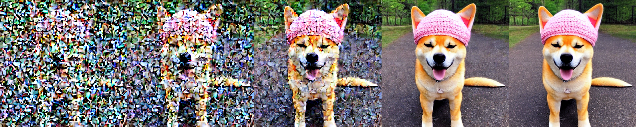
1. User inputs a text prompt, such as “dog with a hat”
2. The text prompt is embedded by a model like CLIP
3. The Diffusion process starts, initialized with random noise (random pixels).
4. The CLIP model compares the embedding of the diffusion model (random pixels) with the text embedding. Uses cosine similarity to compare the two embeddings.
5. The CLIP model backpropagates the loss (the cosine similarity) to the image encoder of the CLIP model, which gives us a gradient of how the pixels should change to make the image more similar to the text prompt.
6. This gradient is used by the diffusion model to generate a new image which is slightly more similar to the text prompt.
7. Repeat steps 4-6 for a number of iterations, which produces an image that is more and more similar to the text prompt.

Exploring CLIP Latent Space

As we can see from the section above, the only part that the user is able to control is the text prompt. The rest of the process is completely black box.

Instead of adjusting the text prompt directly for example changing the prompt to “dog with a blue hat”, what if we could adjust CLIP’s internal representation of “dog with a hat” and add the concept of “blue” to it? Tweaking CLIP’s latent space could potentially give us more fine-grained control over the image generation process.

To start, we need to first figure out how CLIP encodes certain concepts into its latent space. For example, if we want to figure out how CLIP represents the concept of “fatness”, we can generate 100s of prompts with the word “fat” in them, and see where those vectors land in the latent space. Then, we can generate 100s of prompts with the word “thin”, which is semantically the opposite of “fat”, and see where those vectors land. Finally, by taking the average diff between the “fat” and “thin” embeddings, we get a vector that vaguely represents the concept of “fatness”.

MEDIUMS = [
        "painting",
        "drawing",
        "photograph",
        "HD photo",
        "illustration",
        "portrait",
        "sketch",
        "3d render",
        "digital painting",
        "concept art",
        "screenshot",
        "canvas painting"]
SUBJECTS = [
        "dog",
        "cat",
        "horse",
        "ant",
        "ladybug",
        "person",
        "man",
        "woman",
        "child",
        "baby",
        "boy",
        "girl"]
medium = random.choice(MEDIUMS)
subject = random.choice(SUBJECTS)
pos_prompt = f"a {medium} of a {target_word} {subject}"
neg_prompt = f"a {medium} of a {opposite} {subject}"

This code generates a bunch of random prompts, for example “a painting of a fat dog” and “a screenshot of a thin girl”. Then, we can embed these prompts into the CLIP latent space, and take the average diff between the embeddings. Concretely, the function looks like this:

    def find_latent_direction(self,
                              target_word:str,
                              opposite:str):
        with torch.no_grad():
            positives = []
            negatives = []
            for i in tqdm(range(self.iterations)):
                medium = random.choice(MEDIUMS)
                subject = random.choice(SUBJECTS)
                pos_prompt = f"a {medium} of a {target_word} {subject}"
                neg_prompt = f"a {medium} of a {opposite} {subject}"

                print(pos_prompt)
                print(neg_prompt)
                pos_toks = self.pipe.tokenizer(pos_prompt,
                                               padding="max_length",
                                               max_length=self.pipe.tokenizer_max_length,
                                               truncation=True,
                                               return_overflowing_tokens=False,
                                               return_length=False,
                                               return_tensors="pt",).input_ids
                neg_toks = self.pipe.tokenizer(neg_prompt,
                                               padding="max_length",
                                               max_length=self.pipe.tokenizer_max_length,
                                               truncation=True,
                                               return_overflowing_tokens=False,
                                               return_length=False,
                                               return_tensors="pt",).input_ids
                pos = self.pipe.text_encoder(pos_toks).pooler_output
                neg = self.pipe.text_encoder(neg_toks).pooler_output

                positives.append(pos)
                negatives.append(neg)

        positives = torch.cat(positives, dim=0)
        negatives = torch.cat(negatives, dim=0)

        diffs = positives - negatives

        avg_diff = diffs.mean(0, keepdim=True)
        return avg_diff

Then, we can start generating images with our new “fatness” vector. We do so by having a base prompt, for example “a full-body picture of a woman”, embedding it, then adding our fatness vector to it, before passing it into the diffusion model. We can also scale the fatness vector, to create multiple points along the vector that we can use for image generation.

pooled_prompt_embeds = pooled_prompt_embeds + self.avg_diff * scale

Finally, we can generate images with the new prompt, and see how the images change as we scale the fatness vector.

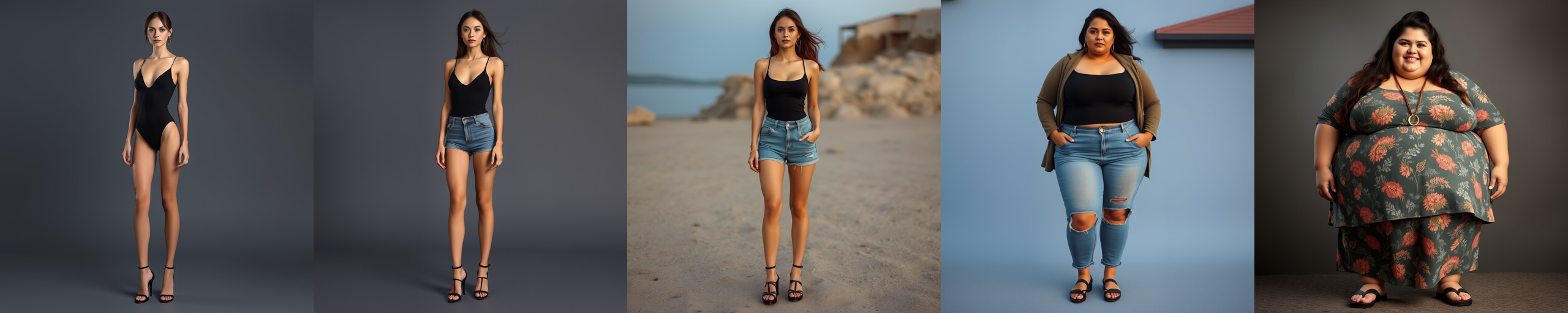
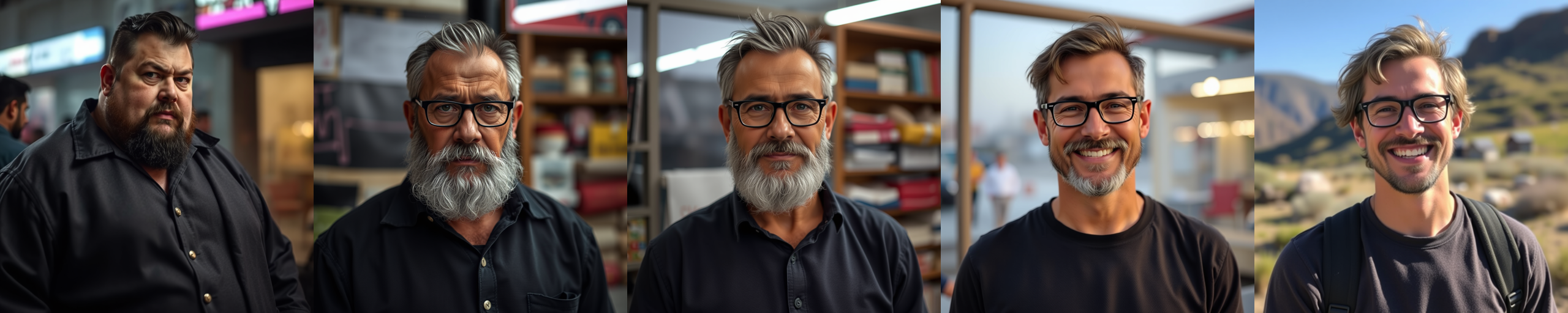
As we can see, this accurately captures the concept of “fatness” in a spectrum from fat to skinny, which we would not have been able to do with prompting alone. However, we also see that the images are not identical, the background and the person’s facial features change as well. This is because our “fatness” vector is not perfect and captures a bunch of unrelated features as well.

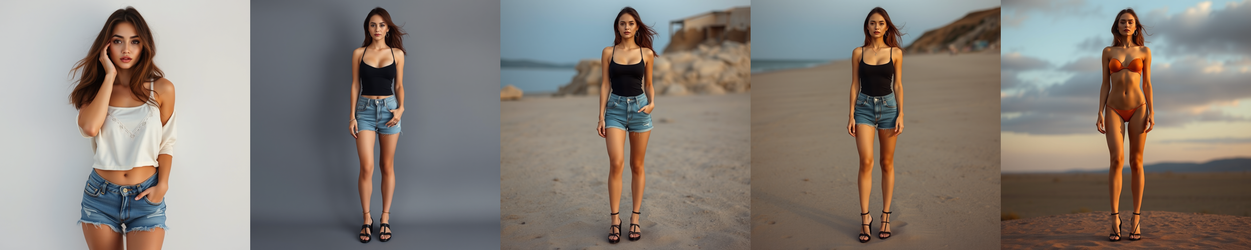
We can repeat the same experiment for “tall” and “short”. This does a slightly worse job at isolating the concept of “tallness”, but still does capture the concept to some degree.

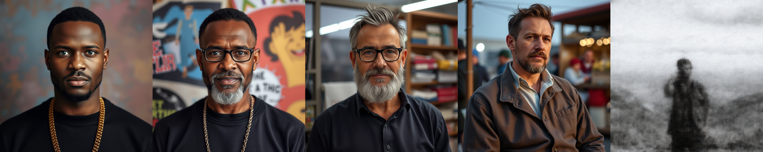
For the “black-white vector”, we can see that the images are not identical, and the last image makes no sense at all. Again, this highlights the imperfection of the method in isolating features.

We don’t need to use opposites to isolate features either. In this example, I used “fat” and “happy” prompts, which did indeed capture the fat/happy spectrum, but again contained a bunch of unrelated features.

Note that for all the images above, the middle image is where the vector is scaled to zero, which means that the vector is not applied. You can see that the middle image is identical, since no additional vector was applied in the first two and the second two examples.

Image Gen & Mechanistic Interpretability

By understanding the internals of neural networks, we may be able to better understand how to control image generation. In the future, one could imagine that these image gen tools will have various sliders and knobs to tweak various parts of the image without trying to specify what you want through text prompts.

The application of Sparse Autoencoders to this use case could be very interesting. Simplistically, sparse autoencoders “expand” the latent space by adding additional dimensions to the neural net, which lets us more easily isolate and control specific features in the image generation process.

I’ll be exploring more on this in a future post, once I top up my GPU credits, stay tuned!